Time
- ΣT ≡ √N = 16 s = measurement duration = sample range
ΣT = 𝚺1..NΔT = N∙ΔTso ΔT is now determined as:
- ΔT = ΣT / N = 1/16 s = sampling interval 𝑇s = time resolution
Display
It is physically intuitive to treat time as one-sided, running from zero (start of measurement) to ΣT (end of measurement) in steps of ΔT.
Human-readable displays usually show time as one-sided. There is no requirement that the last half of the samples be zero. The display above starts the signal at time zero, and draws more than two full measurement durations.
- The one-sided time range 0..16 s is shaded blue (real) or red (imaginary) on some example signals.
However...you will find when entering custom functions that it does indeed matter which range you use. Try this experiment.
- Tap the button to generate an expression for a familiar function of time
- Tap the button to generate the signal and spectrum
- Tap the button to generate the signal and spectrum
- Tap the button to get another function
- Repeat steps 2 and 3
At this point the we switch over to the other column for steps 3 and 4. The half-values are so directly dependent on the full values that they come as afterthoughts.
The half-value
This is primarily just for symmetry in the equations.
- QT = ΣT / 2 = 8 s
One is tempted to call this the “Nyquist” time 𝑇𝑁, but it depends on how you want the analogy to work. If you want it to mean the time beyond which the signal must be zero,” then 𝑇𝑁 should be the measurement duration ΣT = 16 s.
Two-sided time
When drawing a sampled (hence implicitly periodic) time domain as literally circular, it is natural to treat the “last” samples as being in negative time, although events in the “negative half” did not really precede events in the positive half.
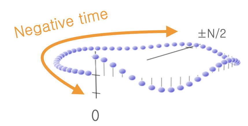
- Some smoothing functions are extended (in lighter gray) to the two-sided time range -8..8 s.
Frequency
The reciprocal of 𝑇s from step 2 must be 𝐹s:
- ΣF = 1 / ΔT = 16 Hz = sample rate 𝐹s= measurement bandwidth
ΣF = 𝚺1..NΔF = N∙ΔFso ΔF is derived as:
- ΔF = ΣF / N = 1/16 Hz = frequency resolution
Display
It is less plausible to treat frequency as one-sided, running from zero (DC) to ΣF.
Human-readable spectra usually omit the redundant bins, or display them as two-sided. When the signals are real, the spectra have even magnitude. The display above centers the frequency at zero, and draws more than two full measurement durations.
- The two-sided frequency range -8..8 Hz is shaded blue (real) or red (imaginary) on some example signals.
The half-value
This is important enough for its own name and symbol
- QF = ΣF / 2 = 8 Hz = 𝐹𝑁 = Nyquist frequency
It is a prerequisite for unambiguous sampling that a signal have no components above 𝐹𝑁. The spectrum values that a DFT provides in the “high half” do not represent beyond-Nyquist frequencies, but negative frequencies paired with positive ones. The information in N real samples is the same as in N/2 complex spectral values.
This apparent asymmetry between the domains’ internal symmetry can be avoided by using the Cosine or Hartley transform.
Two-sided frequency
Drawing a sampled (implicitly periodic) frequency domain as literally circular poses fewer conceptual blocks, because the idea of negative frequency does not seem to raise issues of causality.
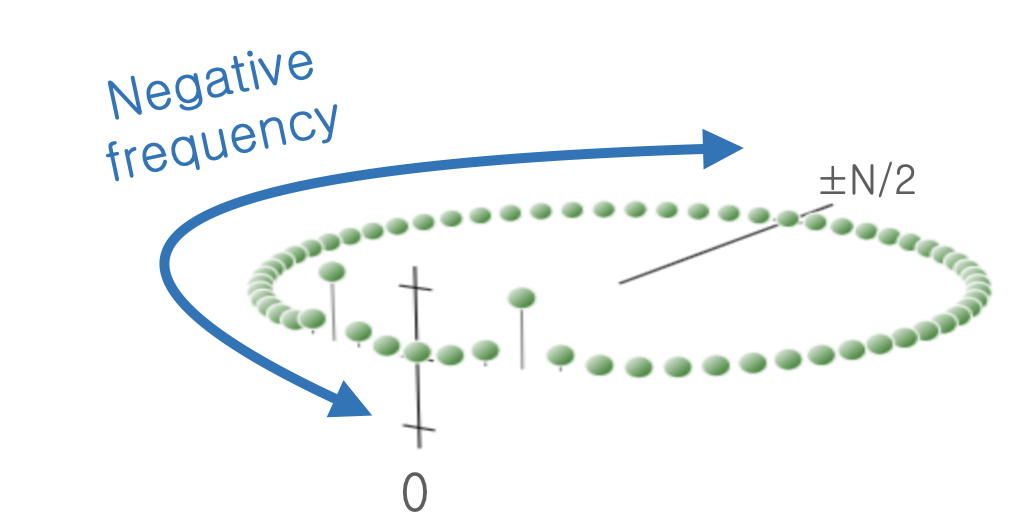
- Smoothing functions are shown over the two-sided frequency range -8..8 Hz.